TODO remove this section
Different solvers solve problems in different ways. Each type has advantages and disadvantages. We 'll roughly discuss a few of the solver types here. You can safely skip this section.
Simplex is an algorithm to find the numerical solution of a linear programming problem.
Advantages:
It knows when it has found an optimal solution.
Disadvantages:
It's complex and mathematical to implement constraints.
Drools Planner does not implement simplex.
Advantages:
It's scalable.
Given a limited time, it can still deliver a pretty decent solution.
Disadvantages:
It does not know when it has found an optimal solution.
If the optimal score is unknown (which is usually the case), it must be told when to stop looking (for example based on time spend, user input, ...).
The genetic algorithm is currently not implemented in Drools Planner.
Local search starts from an initial solution and evolves that single solution into a mostly better and better solution. It uses a single search path of solutions, not a search tree. At each solution in this path it evaluates a number of moves on the solution and applies the most suitable move to take the step to the next solution.
Local search works a lot like a human planner: it uses a single search path and moves facts around to find a good feasible solution.
A simple local search can easily get stuck in a local optima, but improvements (such as tabu search and simulated annealing) address this problem.
Advantages:
It's relatively simple and natural to implement constraints (at least in Drools Planner's implementation).
It's very scalable, even when adding extra constraints (at least in Drools Planner's implementation).
Given a limited time, it can still deliver a pretty decent solution.
Disadvantages:
It does not know when it has found an optimal solution.
If the optimal score is unknown (which is usually the case), it must be told when to stop looking (for example based on time spend, user input, ...).
Drools Planner implements local search, including tabu search and simulated annealing.
As a planning problem gets bigger, the search space tends to blow up really fast. It's not uncommon to see that it's possible to optimally plan 5 people in less then a second, while planning 6 people optimally would take years. Take a look at the problem size of the examples: many instances have a lot more possible solutions than the minimal number of atoms in the known universe (10^80).
The cold, hard reality is that for most real-world planning problems we will not find the optimal solution in our lifetimes. But that's OK, as long as we do better than the solutions created by human planners (which is easy) and other software.
Planning competitions (such as the International Timetabling Competition) show that local search variations (tabu search, simulated annealing, ...) usually perform best for real-world problems given real-world time limitations.
Solving a planning problem with Drools Planner consists out of 4 steps:
Build a solver, for example a tabu search solver for any NQueens puzzle.
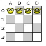
Set a starting solution on the solver, for example a 4 Queens puzzle instance.
Solve it.
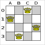
Get the best solution found by the solver.
Every build-in solver implemented in Drools Planner implements the Solver interface:
public interface Solver {


    void setStartingSolution(Solution solution);


    Solution getBestSolution();


    void solve();


    // ...


}
There is normally no need to implement the Solver interface yourself.
A Solver should only be accessed from a single thread, except for the methods that are
specifically javadocced as thread-safe.
You can build a Solver instance with the XmlSolverConfigurer. Configure
it with a solver configuration XML file:
    XmlSolverConfigurer configurer = new XmlSolverConfigurer();

    configurer.configure("/org/drools/planner/examples/nqueens/solver/nqueensSolverConfig.xml");

    Solver solver = configurer.buildSolver();
A basic solver configuration file looks something like this:
<?xml version="1.0" encoding="UTF-8"?>

<localSearchSolver>

    <scoreDrl>/org/drools/planner/examples/nqueens/solver/nQueensScoreRules.drl</scoreDrl>

    <scoreDefinition>

        <scoreDefinitionType>SIMPLE</scoreDefinitionType>

    </scoreDefinition>

    <termination>

        <scoreAttained>0</scoreAttained>

    </termination>

    <selector>

        <moveFactoryClass>org.drools.planner.examples.nqueens.solver.NQueensMoveFactory</moveFactoryClass>

    </selector>

    <acceptor>

        <completeSolutionTabuSize>1000</completeSolutionTabuSize>

    </acceptor>

    <forager>

        <pickEarlyType>NEVER</pickEarlyType>

    </forager>

</localSearchSolver>
This is a tabu search configuration for n queens. We 'll explain the various parts of a configuration later in this manual.
Drools Planner makes it relatively easy to switch a solver type just by changing the configuration. There's even a benchmark utility which allows you to play out different configurations against each other and report the most appropriate configuration for your problem. You could for example play out tabu search versus simulated annealing, on 4 queens and 64 queens.
A solver has a single Random instance. Some solver configurations use the
Random instance a lot more than others. For example simulated annealing depends highly on
random numbers, while tabu search only depends on it to deal with score ties. The environment mode influences the
seed of that Random instance.
The environment mode also allows you to detect common bugs in your implementation.
You can set the environment mode in the solver configuration XML file:
<localSearchSolver>

    <environmentMode>DEBUG</environmentMode>

    ...

</localSearchSolver>
There are 4 environment modes:
The trace mode is reproducible (see the reproducible mode) and also turns on all assertions (such as assert that the delta based score is uncorrupted) to fail-fast on rule engine bugs.
The trace mode is very slow (because it doesn't rely on delta based score calculation).
The debug mode is reproducible (see the reproducible mode) and also turns on most assertions (such as assert that the undo Move is uncorrupted) to fail-fast on a bug in your Move implementation, your score rule, ...
The debug mode is slow.
It's recommended to write a test case which does a short run of your planning problem with debug mode on.
The reproducible mode is the default mode because it is recommended during development. In this mode, 2 runs on the same computer will execute the same code in the same order. They will also yield the same result, except if they use a time based termination and they have a sufficiently large difference in allocated CPU time. This allows you to benchmark new optimizations (such as a new move implementation or a different minimalAcceptedSelection setting) fairly.
The reproducible mode is not much slower than the production mode.
In practice, this mode uses the default random seed, and it also disables certain concurrency optimizations (such as work stealing).
The production mode is the fastest and the most robust, but not reproducible. It is recommended for a production environment.
The random seed is different on every run, which makes it more robust against an unlucky random seed. An unlucky random seed gives a bad result on a certain data set with a certain solver configuration. Note that in most use cases the impact of the random seed is relatively low on the result (even with simulated annealing). An occasional bad result is far more likely caused by another issue (such as a score trap).
A Solver can only solve 1 problem instance at a time.
You need to present the problem as a starting Solution instance to the solver.
You need to implement the Solution interface:
public interface Solution<S extends Score> {


    S getScore();

    void setScore(S score);


    Collection<? extends Object> getFacts();


    Solution<S> cloneSolution();


}
For example, an NQueens instance just holds a list of all its queens:
public class NQueens implements Solution<SimpleScore> {


    private List<Queen> queenList;


    // ...


}
A Solution requires a score property. The score property is null if the
Solution is uninitialized or if the score has not yet been (re)calculated. The score property
is usually typed to the specific Score implementation you use. For example,
NQueens uses a SimpleScore:
    private SimpleScore score;


    public SimpleScore getScore() {

        return score;

    }


    public void setScore(SimpleScore score) {

        this.score = score;

    }
Most use cases use a HardAndSoftScore instead.
All objects returned by the getFacts() method will be asserted into the drools working
memory. Those facts can be used by the score rules. For example, NQueens just returns all
Queen instances.
    public Collection<? extends Object> getFacts() {

        return queenList;

    }
Most solvers use the cloneSolution() method to clone the solution each time they
encounter a new best solution. The NQueens implementation just clones all
Queen instances:
    public NQueens cloneSolution() {

        NQueens clone = new NQueens();

        List<Queen> clonedQueenList = new ArrayList<Queen>(queenList.size());

        for (Queen queen : queenList) {

            clonedQueenList.add(queen.clone());

        }

        clone.queenList = clonedQueenList;

        clone.score = score;

        return clone;

    }
The cloneSolution() method should clone no more and no less than the parts of the
Solution that can change during planning. For example, in the curriculum course schedule
example the lectures are cloned, but teachers, courses, timeslots, periods, rooms, ... are not cloned because only
a lecture's appointed period or room changes during solving:
    /**

     * Clone will only deep copy the {@link #lectureList}.

     */

    public CurriculumCourseSchedule cloneSolution() {

        CurriculumCourseSchedule clone = new CurriculumCourseSchedule();

        ...

        clone.teacherList = teacherList;

        clone.curriculumList = curriculumList;

        clone.courseList = courseList;

        clone.dayList = dayList;

        clone.timeslotList = timeslotList;

        clone.periodList = periodList;

        clone.roomList = roomList;

        clone.unavailablePeriodConstraintList = unavailablePeriodConstraintList;

        List<Lecture> clonedLectureList = new ArrayList<Lecture>(lectureList.size());

        for (Lecture lecture : lectureList) {

            Lecture clonedLecture = lecture.clone();

            clonedLectureList.add(clonedLecture);

        }

        clone.lectureList = clonedLectureList;

        clone.score = score;

        return clone;

    }
First, you will need to make a starting solution and set that on the solver:
solver.setStartingSolution(startingSolution);
For 4 queens we use a simple filler algorithm that creates a starting solution with all queens on a different x and on the same y (with y = 0).
Here's how we generate it:
    private NQueens createNQueens(int n) {

        NQueens nQueens = new NQueens();

        nQueens.setId(0L);

        List<Queen> queenList = new ArrayList<Queen>(n);

        for (int i = 0; i < n; i++) {

            Queen queen = new Queen();

            queen.setId((long) i);

            queen.setX(i); // Different column

            queen.setY(0); // Same row

            queenList.add(queen);

        }

        nQueens.setQueenList(queenList);

        return nQueens;

    }
The starting solution will probably be far from optimal (or even feasible). Here, it's actually the worst possible solution. However, we 'll let the solver find a much better solution for us anyway.
Solving a problem is quite easy once you have a solver and the starting solution:
    solver.setStartingSolution(startingSolution);

    solver.solve();

    Solution bestSolution = solver.getBestSolution();
The solve() method will take a long time (depending on the problem size and the solver
configuration). The solver will remember (actually clone) the best solution it encounters during its solving.
Depending on a number factors (including problem size, how long you allow the solver to work, which solver type you
use, ...), that best solution will be a feasible or even an optimal solution.
After a problem is solved, you can reuse the same solver instance to solve another problem (of the same problem type).

